The Sharpe Ratio

Balancing Risk and Reward: A Dive into the Sharpe Ratio for Beginner Investors

What is the Sharpe Ratio?

The Sharpe Ratio tells you how much extra return you’re earning for every unit of risk you take. The "extra return" is the amount you earn above a super-safe investment, like a government bond or Treasury bill (often called the "risk-free rate"). The "risk" part is how much the investment’s value bounces around (volatility), measured by something called standard deviation.

---

How Useful Is It?

The Sharpe Ratio is handy for comparing investments or portfolios. A higher Sharpe Ratio means better risk-adjusted returns—more bang for your buck in terms of risk. It’s widely used by investors to:

• Assess whether an investment’s returns justify its risk.

• Compare different assets or strategies (e.g., stocks vs. bonds).

• Optimize portfolios by favoring higher Sharpe Ratios.

Limitations:

• It assumes returns are normally distributed (which isn’t always true—think crashes or fat tails).

• It doesn’t distinguish between upside and downside risk (volatility can come from gains, not just losses).

• It’s less useful for assets with non-linear returns (like options).

---

How to Calculate the Sharpe Ratio

The Sharpe Ratio is a measure used to evaluate the risk-adjusted return of an investment or portfolio. It tells you how much excess return you’re getting for each unit of risk you’re taking. Here’s the formula:

Sharpe Ratio = (Rp - Rf) / σp

Where:

• Rp = Expected portfolio return (average return of the investment)

• Rf = Risk-free rate (e.g., return on risk-free asset such as a government bond)

• σp = Standard deviation of the portfolio’s excess return (a measure of how wild the ups and downs of the investment are)

Steps:

1. Determine Rp: Calculate the average return of your portfolio over a specific period (e.g., annualized return).

2. Find Rf: Identify the risk-free rate for the same period.

3. Calculate Excess Return: Subtract Rf from Rp (this is the return above the risk-free rate).

4. Compute σp: Calculate the standard deviation of the portfolio’s returns to measure its volatility.

5. Divide: Divide the excess return by the standard deviation to get the Sharpe Ratio.

---

Illustrative Example

In this example, I will provide approximate figures for my TFSA portfolio, which commenced in 2019. For further context, please to my previously published post below.

Step 1: Portfolio Annualized Return (Rp)

Identify your annualized return. For this instance, the annualized return of this portfolio was 11.55% over the period from 2019 to 2024.

Step 2: Risk-Free Rate (Rf​)

Estimate the average risk-free rate over the referenced time period (2019 to 2024). As a Canadian investor, typically, the risk-free rate is approximated using short-term government securities, like the 1-month or 3-month Canadian Treasury bills, or sometimes the Bank of Canada’s target overnight rate as a proxy.

The Bank of Canada provides historical data on Treasury bill yields and overnight rates. Over this period, rates fluctuated significantly due to economic conditions:

• 2019: Rates were around 1.5–1.75% (pre-COVID, relatively stable).

• 2020: Rates dropped sharply to near 0% (around 0.25%) due to COVID-19 stimulus.

• 2021: Rates remained low, around 0.25%.

• 2022: Rates rose as the Bank of Canada hiked rates to combat inflation, averaging around 2–3% by year-end.

• 2023: Rates continued to rise, peaking around 5% for the overnight rate.

• 2024: Rates began to ease slightly but stayed elevated, likely averaging around 4–5%.

For simplicity, we can approximate the average risk-free rate over the 6-year period. A rough estimate, based on historical trends, might be around 2–3% annualized, reflecting low rates early in the period and higher rates later. For this example, 2.5% is used as a reasonable average for the risk-free rate.

Step 3: Standard Deviation of Annual Returns (σp)

Calculate the standard deviation of the annual returns to measure volatility.

The annual returns are:

• 2019: 3.58%

• 2020: 10.57%

• 2021: 24.83%

• 2022: -9.78%

• 2023: 22.20%

• 2024: 7.62%

Compute the mean of these annual returns:

Next, compute the variance by finding the squared differences from the mean, summing them, and dividing by n−1:

Calculate each squared difference:

Sum the squared differences:

Divide by n−1 (i.e. 6-1=5) and calculate the variance:

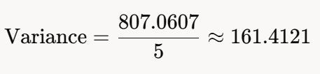
Take the square root to get the standard deviation:

So, the standard deviation of these annual returns is approximately 12.70%.

Step 4: Calculate the Sharpe Ratio

Using the values that have been calculated:

Rounding to two decimal places, the Sharpe ratio of this portfolio as at the end of 2024 was approximately 0.71.

---

General Benchmarks and Caveats

In general, a Sharpe ratio:

• Below 1 is considered subpar.

• Between 1 and 2 is good.

• Above 2 is excellent.

But other considerations are important as well:

Asset Class and Investment Strategy

• Different asset classes and strategies have different expected Sharpe ratios due to their inherent risk-return profiles.

  • Equities: Equity portfolios typically target a Sharpe ratio of 0.5 to 1.5, depending on market conditions. A ratio above 1.0 is often considered good for stocks because of their higher volatility.

  • Fixed Income: Bond portfolios tend to have lower volatility and lower returns, so their Sharpe ratios might range from 0.2 to 1.0. A ratio above 0.5 can be good for bonds.

  • Hedge Funds/Alternatives: Some hedge funds or alternative strategies aim for higher Sharpe ratios (1.5 to 3.0) because they often employ leverage or target absolute returns.

Time Period

• The time frame over which the Sharpe ratio is calculated matters. Short-term ratios can be skewed by outliers or temporary market conditions, while longer-term ratios (e.g., 5–10 years) provide a more reliable picture.

Comparison to Benchmarks and Peers

• A Sharpe ratio should be compared to relevant benchmarks or peer portfolios.

  • Compare an equity portfolio to a broad market index like the S&P 500 or TSX Composite.

Investor Goals and Risk Tolerance

• What is considered "good" depends on investor’s objectives. A risk-averse investor may prefer a lower Sharpe with volatility, whereas a risk tolerant investor might accept a lower Sharpe ratio for the opportunity of higher absolute returns.

---

Overall Conclusion

Given the short time period of this portfolio, where investments only started to ramp up in 2022, the Sharpe ratio of 0.71 can be skewed by a few outliers. More investing years need to be accounted for to determine a less sensitive ratio. However, this small analysis reveals that my risk tolerance has been more risk-averse. As this portfolio’s strategy continues to evolve, it will take a few more years for this ratio to evolve and better reflect the portfolio’s risk.

From a benchmark perspective, the Sharpe ratio was roughly estimated for the major indices in the U.S. and Canada as follows:

• S&P 500 - 0.85

• S&P/TSX Composite - 0.69

• Portfolio - 0.71

This example was intended to illustrate the Sharpe ratio and its calculation method. Ultimately, investors prioritize total returns, and the Sharpe ratio serves as one of many tools that can provide insight, though it doesn’t capture the full picture. While it remains a useful metric for evaluating risk-adjusted performance, it’s best utilized alongside other measures and qualitative considerations to gain a well-rounded understanding of an investment’s overall performance.

---

● Written with the help of Grok

Consider joining DiviStock Chronicles’ Referral Program for more neat rewards!

Please refer to the details of the referral program.